Convolutional Neural Networks: LeNet-5 and LeCun et al. (1998)
How convolution, shared weights, and pooling made LeNet-5 practical for image recognition and shaped modern computer vision.
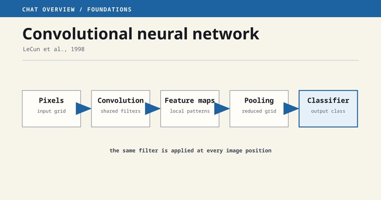
Convolutional neural networks, usually shortened to CNNs, are neural networks designed for data with a regular spatial structure. Instead of connecting every image pixel to a separate weight, a CNN learns small filters and applies each filter across the image.
This arrangement builds two assumptions into the model. Nearby pixels are likely to form meaningful local patterns, and a useful pattern can appear in more than one location. The assumptions are called inductive biases: they limit the set of possible computations in a way that suits the problem.
Yann LeCun and collaborators developed convolutional systems over many years. Their 1998 paper Gradient-Based Learning Applied to Document Recognition presented LeNet-5 and a complete system for reading handwritten checks. It is a useful landmark because it joins architecture, backpropagation , data preparation, and deployment into one engineering account.
Historical Context
Kunihiko Fukushima's neocognitron, published in 1980, used alternating stages of feature extraction and tolerance to small spatial changes. LeCun's early work added supervised gradient-based training to related ideas. By the late 1980s, convolutional networks could recognize handwritten ZIP codes.
A fully connected network treats each pixel position as unrelated to every other position. For a modest image, this produces a large parameter count and fails to express a fact a vision engineer already knows: an edge is an edge whether it is near the top or bottom of the frame.
CNNs address this with three recurring ideas:
- Local receptive fields: a unit reads a small neighborhood rather than the entire image.
- Shared weights: the same filter is used at every valid location.
- Spatial reduction: pooling or strided operations reduce resolution as features become more abstract.
Weight sharing reduces parameters and makes the response equivariant to translation: if the input feature moves, the corresponding feature-map response moves. Pooling and later processing can make the final classification less sensitive to small movements. It is more accurate to say "translation tolerance" than to claim that every CNN is perfectly translation invariant.
How Convolution Works
Take a small grid of weights, perhaps 3 by 3. Place it over one patch of the image. Multiply corresponding values, add the products and a bias, and record the result. Move the filter to the next position and repeat. The resulting grid is a feature map.
During training, the filter weights change. One filter may become sensitive to a horizontal edge, another to a texture, and another to a color transition. These descriptions are useful intuition, not predefined roles. The filters learn whatever lowers the loss.
An input may have several channels, such as red, green, and blue. A filter spans all input channels and produces one output channel. A convolutional layer learns many filters, so its output is a stack of feature maps.
Several settings determine the shape:
- Kernel size is the filter's spatial width and height.
- Stride is the distance the filter moves between applications.
- Padding adds values around the border, often to preserve size.
- Dilation spaces kernel elements apart to enlarge the receptive field.
Despite the name, deep-learning libraries commonly calculate cross-correlation rather than mathematically flipping the kernel as a strict convolution would. Because the weights are learned, this convention does not reduce the layer's usefulness.
Nonlinearity and Pooling
Stacking linear convolutions without activation functions would still describe one linear transformation. An activation function such as the rectified linear unit, or ReLU, makes the network nonlinear. ReLU returns zero for negative inputs and the input itself for positive values.
Pooling replaces a local region with a summary. Max pooling keeps the largest value; average pooling keeps the mean. LeNet-5 used trainable subsampling layers. Later networks often use max pooling or strided convolutions.
As layers accumulate, each output depends on a larger region of the original image. This effective region is the receptive field. Early layers can respond to local structure; later layers combine those responses across broader areas.
LeNet-5
LeNet-5 accepts a 32 by 32 grayscale image and passes it through alternating convolutional and subsampling stages. The spatial dimensions shrink while the number of feature maps grows. Final fully connected stages produce ten outputs for digit classes.
The 1998 paper is broader than this diagram. It describes graph transformer networks that combine trainable modules with constraints for document recognition. In the deployed check-reading system, segmentation, recognition, and language-level constraints worked together. LeNet-5 was therefore a key component of a practical system, not an isolated benchmark trick.
The network was trained end to end. Backpropagation calculated gradients for shared filter weights just as it did for ordinary weights. Sharing requires gradient contributions from every place where a filter was applied to be accumulated into the same parameter update.
Impact and Applications
CNNs were commercially useful for document reading before they dominated academic computer vision. Their broader rise depended on larger labeled datasets, faster hardware, improved optimization, and deeper designs.
AlexNet's 2012 ImageNet result made that combination impossible to ignore. VGG explored depth with small filters. Inception used parallel branches at different scales. ResNet added skip connections that made very deep networks easier to train. EfficientNet studied coordinated scaling of width, depth, and input resolution.
CNNs became standard components for image classification, object detection, segmentation, medical imaging, remote sensing, audio spectrograms, and scientific grids. They also served as encoders in encoder-decoder systems and as the visual backbone of early multimodal models.
Vision Transformers now compete with or replace CNNs in many large-scale systems. The change does not make convolution irrelevant. CNNs remain efficient, are often easier to deploy on limited hardware, and encode a useful local bias when data is scarce.
Limits and Failure Modes
The assumptions that help a CNN can also constrain it. Local filters do not directly model distant relationships. Deep stacks, dilation, or attention are needed to connect far-apart regions. Standard convolutions also do not automatically handle rotation, scale changes, or perspective.
Downsampling can discard precise location information. Classification benefits from tolerance to small shifts, while segmentation and keypoint tasks need exact spatial output. Skip connections and feature pyramids help preserve detail.
Finally, high benchmark accuracy does not imply reliable perception. CNNs can depend on texture, background correlations, or dataset artifacts. Include shifted conditions and task-specific failure analysis in the evaluation.
A Practical Reading of the Architecture
The durable lesson of CNNs is not that every vision system must use convolution. It is that an architecture can represent known structure in the data. Shared local filters made learning more data-efficient and computationally manageable. Later architectures make different tradeoffs, but the engineering principle remains.
Related Work
- The Perceptron explains a trainable linear classifier without spatial weight sharing.
- Backpropagation supplies the training method used by LeNet.
- Encoder-Decoder Models use CNNs when the source is an image or spatial field.
- Transformers provide an alternative based on attention.
Further Reading
- Tags:
- Papers
- Architectures