The Perceptron: Rosenblatt (1958)

How Rosenblatt's perceptron learns a linear decision boundary, why convergence has conditions, and where the model fails.

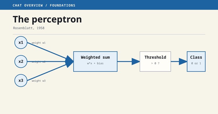
By Chat Overview Published August 5, 2025 Updated September 1, 2026

A perceptron weights its inputs, adds a bias, and applies a threshold to choose between two classes.

The perceptron is a trainable binary classifier. It multiplies each input by a learned weight, adds the results and a bias, then applies a threshold. Frank Rosenblatt presented the model in his 1958 paper, "The Perceptron: A Probabilistic Model for Information Storage and Organization in the Brain."

The model is small enough to calculate by hand, but it introduced a durable pattern: choose a parameterized function, compare its prediction with a known label, and change the parameters after an error. Modern neural networks use richer units and a different training procedure, yet that basic separation between a forward calculation and a learning rule remains.

The perceptron has a strict limit. One unit can learn only a linear decision boundary. If no straight line, plane, or higher-dimensional hyperplane separates the classes, the perceptron learning algorithm will not find a stable solution.

Historical context

The 1958 paper sits between early mathematical models of neurons and later machine-learning systems. Warren McCulloch and Walter Pitts had described networks of simplified threshold units in 1943. Donald Hebb's 1949 work discussed changes in connection strength through experience. Rosenblatt tried to turn related ideas into a system that learned associations from examples.

The paper describes a broader perceptron system than the compact classroom algorithm normally called "the perceptron" today. It includes sensory units, association units, response units, random connections, and learning rules. Rosenblatt framed the work as a model for perception and memory, not merely as a convenient linear classifier.

The Mark I Perceptron later implemented parts of the approach in hardware. Its visual demonstrations helped make trainable machines a public subject. When reading historical accounts, keep the paper, the Mark I hardware, and the modern simplified algorithm distinct.

The modern calculation

Let the input be a vector x, the weights be a vector w, and the bias be b. The perceptron first calculates a score:

score = w dot x + b

It then applies a step function. One common convention returns class 1 when the score is greater than or equal to zero and class 0 otherwise.

The weights define the orientation of the decision boundary. The bias moves that boundary without changing its orientation. In two input dimensions, the boundary is a line. In three dimensions it is a plane. The same idea extends to more dimensions even though it cannot be drawn directly.

Suppose the inputs are x1 = 2 and x2 = 1, the weights are w1 = 0.6 and w2 = -0.4, and the bias is -0.3. The score is:

(0.6 * 2) + (-0.4 * 1) - 0.3 = 0.5

With a zero threshold, the output is class 1. This result explains the current prediction. It does not show whether the weights are good; that requires labeled examples not used to calculate this single output.

The learning rule

Training processes labeled examples. For an input x, expected label y, and prediction prediction, calculate the error:

error = y - prediction

Then update each weight using a learning rate rate:

w = w + rate * error * x

The bias receives a corresponding update:

b = b + rate * error

If the prediction is correct, the error is zero and no update is made. If a positive example is classified as negative, its input vector is added to the weights. If a negative example is classified as positive, its input vector is subtracted.

This is an online learning rule because it can update after each example. Implementations may iterate through the training set several times. Shuffling the examples can change the path taken through weight space, even when the final boundary classifies all training examples correctly.

What convergence means

The perceptron convergence theorem applies when the training data is linearly separable and the examples satisfy the theorem's assumptions. Under those conditions, repeated updates reach a separating boundary in a finite number of mistakes.

The theorem does not say that:

The returned boundary is unique.
The boundary has the largest possible margin.
The model will generalize to unseen data.
Training will converge when classes overlap or contain contradictory labels.
A low training error proves that the input features are appropriate.

If the data is not linearly separable, the standard learning rule can keep changing the weights. A practical implementation therefore needs a stopping condition such as a maximum number of passes, a held-out score, or a no-improvement threshold.

XOR and linear separability

Exclusive OR, usually written XOR, is the standard counterexample. With two binary inputs, XOR is positive when exactly one input is positive. The points (0,1) and (1,0) belong to one class, while (0,0) and (1,1) belong to the other. No single straight line separates those two groups.

A single perceptron cannot represent XOR. A network with a hidden layer can combine several boundaries to do so. The hidden units transform the input into a representation in which the final decision becomes separable.

This is the conceptual bridge to multilayer networks. The bridge also creates a training problem: the desired labels are known for the output, but not for each hidden unit. Backpropagation supplies gradients that assign part of the output error to those internal parameters.

Minsky and Papert

Marvin Minsky and Seymour Papert analyzed the mathematical capabilities and limits of perceptrons in their 1969 book Perceptrons. The book is often summarized as having ended neural-network research because it showed the XOR limitation. That account is too simple.

The single-layer limitation was real and important, but research funding and interest changed for several technical and institutional reasons. Multilayer networks were also difficult to train with the available methods and computing resources. The later spread of backpropagation, larger datasets, and faster hardware changed that practical situation.

Use the book as an analysis of a model class, not as proof that all neural networks share the same limit.

Relationship to modern neural networks

A modern dense layer still calculates weighted sums and biases, but it normally uses a differentiable activation such as ReLU, sigmoid, or GELU rather than a hard threshold during training. Differentiability allows gradient-based optimization across many layers.

Multiclass systems also use several output units or a structured output distribution instead of one binary response. Convolutional networks share weights across image positions. Recurrent networks reuse weights across time. Transformers calculate context-dependent interactions with attention. These systems are much more than stacked perceptrons, but learned weighted combinations remain a basic operation.

When the perceptron is still useful

The perceptron is useful for teaching because every calculation is visible. It also provides a baseline for linearly separable data and a reference point for online learning.

Do not use it merely because a dataset has two labels. Check whether the feature representation makes a linear boundary plausible, whether class imbalance changes the useful error measure, and whether probability estimates are required. A hard-threshold perceptron does not produce a calibrated probability.

Turing's Computing Machinery and Intelligence asked how to evaluate machine behavior. The perceptron addressed a different question: how a machine could change its response from examples. Backpropagation made multilayer representation learning practical, while convolutional networks added structure suited to images.