Backpropagation: Rumelhart, Hinton, and Williams (1986)
How backpropagation uses the chain rule to train multilayer neural networks, and why the 1986 paper mattered.
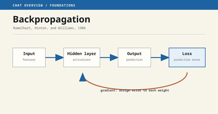
Backpropagation is the standard method for finding out how much each trainable weight contributed to a neural network's error. It works backward from a loss value and applies the chain rule of calculus at every operation in the network.
That description is more precise than saying that backpropagation "learns." Backpropagation computes gradients. An optimizer, such as stochastic gradient descent or Adam, uses those gradients to update the weights. Keeping those two jobs separate makes modern training systems much easier to understand.
The method is associated with David Rumelhart, Geoffrey Hinton, and Ronald Williams because their 1986 paper, Learning representations by back-propagating errors, showed clearly how it could train multilayer networks to form useful internal representations. The underlying mathematical ideas had earlier precedents, but the 1986 work made the method visible, practical, and influential.
Historical Context
The perceptron had a learning rule, but a single perceptron could only learn a linear decision boundary. Multilayer networks were more expressive, yet their hidden units created a practical problem. The desired output was known, but no target value was supplied for each hidden unit. A training procedure needed to assign responsibility for the final error throughout the network.
Reverse-mode differentiation supplied the answer. Work by Seppo Linnainmaa, Paul Werbos, and others established important parts of the method before 1986. Rumelhart, Hinton, and Williams presented it in a form that connectionist researchers could apply to neural networks and backed it with experiments on learned representations.
The timing mattered. Interest in connectionist systems had declined after the limits of single-layer perceptrons became widely understood. Backpropagation did not remove every difficulty in neural-network training, but it made hidden layers trainable by a general procedure. That reopened an architectural path which eventually led to convolutional networks, recurrent networks, and Transformers.
The Training Loop
Training a conventional neural network repeats four steps:
Run a forward pass from the input to the prediction. 2. Compare the prediction with the target using a loss function. 3. Run backpropagation to compute the derivative of the loss with respect to each parameter. 4. Let the optimizer update the parameters.
For a weight w, a simple gradient-descent update is w_new = w - learning_rate * dL/dw.
The derivative dL/dw says how a small change in w is expected to change the loss L.
The minus sign moves the weight in the direction expected to reduce the loss locally.
Backpropagation computes dL/dw; it does not choose the learning rate or batch examples, or determine how an optimizer accumulates momentum.
Those belong to the optimizer and the wider training procedure.
Why the Chain Rule Is Enough
A neural network is a composition of simpler functions.
Suppose an input x is multiplied by w, passed through an activation function, and then used to calculate a loss.
The effect of w on the loss is indirect.
The chain rule breaks that indirect effect into local derivatives:
dL/dw = dL/doutput * doutput/dactivation * dactivation/dw
The backward pass starts with the derivative of the loss at the output. Each operation receives a gradient from the operation after it, multiplies that gradient by its own local derivative, and passes the result backward. When a value affects several later operations, the returning gradient contributions are added.
This reuse is important. Calculating every derivative independently would repeat large parts of the same computation. Reverse-mode differentiation stores the intermediate values from the forward pass, then traverses the resulting computation graph in reverse. It can therefore calculate gradients for millions or billions of parameters with a cost that is a small multiple of the forward computation.
A Small Worked Chain
Consider the deliberately simple model prediction = w * x, with squared error L = (prediction - target)^2.
Let x = 3, target = 10, and w = 2.
The forward pass gives a prediction of 6 and a loss of 16. Working backward:
dL/dprediction = 2 * (prediction - target) = -8dprediction/dw = x = 3dL/dw = -8 * 3 = -24
With a learning rate of 0.01, gradient descent changes the weight from 2 to 2.24. On the same example, the new prediction is 6.72 and the loss is lower. Real networks contain many branches, matrices, and nonlinear functions, but the accounting principle is the same.
What Hidden Layers Learn
A hidden unit is not given a label for a feature to detect. Its gradient depends on how it affects later units and, eventually, the loss. Across many examples, useful intermediate features receive updates that improve the final task.
In an image classifier, early layers may become sensitive to edges while later layers combine those responses into shapes. In a language model, internal representations may encode syntax, reference, or factual associations. These interpretations are approximate, not labels installed by the developer. The training objective rewards whatever internal organization helps reduce loss.
Why the 1986 Paper Mattered
The paper demonstrated more than a derivative calculation. It argued that useful representations could emerge in hidden layers when a network was trained end to end. Its examples included learning family relationships and encoding the structure of words. This supported a different way to build intelligent systems: specify an objective and a differentiable architecture, then let training discover intermediate features.
The method also provided a common training mechanism across different architectures. Convolutional neural networks use local connectivity and shared weights. LSTMs add gated recurrent state. Transformers use attention. All can be represented as differentiable computations and trained with backpropagation.
Common Training Problems
Backpropagation gives correct derivatives for the implemented computation, but correct gradients do not guarantee useful training.
- Vanishing gradients: repeated multiplication by small derivatives can make early layers learn very slowly. LSTM gates, residual connections, careful initialization, and normalization help.
- Exploding gradients: large derivatives can make updates unstable. Gradient clipping is a common safeguard.
- Poor conditioning: the loss surface may be much steeper in some directions than others, which slows optimization.
- Overfitting: a network can minimize training loss without generalizing to unseen data.
- Bad objectives: the network optimizes the stated loss, not the developer's unstated intention.
For small custom operations, gradient checking can catch implementation errors. Perturb a parameter slightly, measure the numerical change in loss, and compare that estimate with the analytical gradient. Numerical estimates are too expensive for training, but useful as a test.
Limits and Misconceptions
Backpropagation is sometimes described as biologically implausible because it assumes precise backward signals and coordinated weights. That criticism concerns it as a model of biological learning, not its effectiveness as an engineering method.
It is also not a guarantee of global optimization. Neural-network losses are non-convex, and gradient methods usually find a useful solution rather than a provably best one. Results depend on the data, architecture, objective, optimizer, initialization, and available computation.
Finally, solving XOR was evidence that a multilayer network could represent a nonlinear boundary. It was not the sole purpose or achievement of the 1986 paper. The durable contribution was a practical, general method for assigning credit through layers of computation.
Related Work
- The Perceptron explains the earlier single-layer learning rule and its limits.
- Long Short-Term Memory addresses gradient flow through recurrent sequences.
- Convolutional Neural Networks apply backpropagation to shared spatial filters.
- Transformers remain trained by backpropagation even though their architecture removes recurrence.
Further Reading
- Tags:
- Papers
- Architectures