Long Short-Term Memory (LSTM): Hochreiter and Schmidhuber (1997)

How LSTM cells use gated state to learn long-range sequence dependencies, and what the 1997 paper actually introduced.

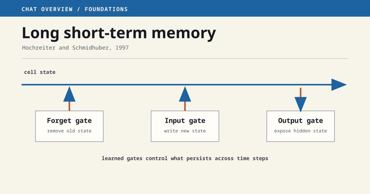
By Chat Overview Published August 5, 2025 Updated September 1, 2026

An LSTM cell controls what to remove, write, and expose while carrying state across time steps.

Long short-term memory, usually shortened to LSTM, is a recurrent neural-network architecture designed to preserve useful error signals across many time steps. Sepp Hochreiter and Jurgen Schmidhuber introduced it in a 1997 paper in Neural Computation.

The core idea is a state path with controlled read and write operations. A standard recurrent network repeatedly transforms its hidden state. An LSTM adds a cell state whose update can remain close to additive. Learned gates decide which information enters that state and which part becomes visible to the rest of the network. This structure makes some long-range dependencies easier to learn with gradient descent.

LSTM did not make long-term memory automatic, and it did not eliminate every vanishing-gradient problem. It gave the optimizer a better route through time. That distinction matters when comparing the paper with later claims about what LSTMs can remember.

The problem with a standard recurrent network

A recurrent neural network processes a sequence one item at a time. At time step t, it combines the current input with the hidden state from time step t-1. The same weights are reused at every step.

Training normally uses backpropagation through time. The network is unfolded into a chain, and the loss gradient is propagated backward through each repeated operation. See Backpropagation for the underlying chain-rule calculation.

The repeated multiplication is the problem. If the relevant derivatives are mostly smaller than one, the gradient shrinks as it travels backward. A distant event then receives almost no useful learning signal. If those derivatives are consistently larger than one, the gradient can grow until training becomes unstable.

The number of units alone does not explain the problem. A larger recurrent state can still fail to learn that an observation near the start of a sequence affects an output much later.

Hochreiter analyzed this long-time-lag problem in earlier work. The 1997 paper proposed an architecture whose internal state could carry error information across a longer interval without repeatedly applying the same shrinking transformation.

The memory cell

The original LSTM design introduced a memory cell with a self-connection. The authors called the protected state path a constant error carousel. Its purpose was to let an error signal circulate without immediately vanishing or exploding.

Two learned gates controlled access:

The input gate controlled whether a new candidate value entered the cell.
The output gate controlled whether the cell affected the visible output.

The widely taught modern LSTM also has a forget gate. That gate scales the previous cell state before the new candidate is added. It lets the network deliberately remove old information. The forget gate was introduced in later work by Felix Gers, Jurgen Schmidhuber, and Fred Cummins, not in the original 1997 architecture.

Modern explanations usually describe the update in four parts:

Compute a forget value between zero and one. 2. Compute an input value and a candidate state. 3. Combine retained old state with gated new state. 4. Compute an output value and expose part of the updated state.

A sigmoid function is commonly used for gates because it returns values between zero and one. A value near zero suppresses a path. A value near one leaves most of it open. The candidate and exposed state commonly use a hyperbolic tangent, which keeps those values in a bounded range.

These descriptions are conventions, not a single immutable specification. Libraries can differ in gate order, bias initialization, projection layers, peephole connections, and naming. Check the implementation before loading weights or comparing parameter counts.

A simple sequence example

Consider a model that reads a log stream and must report whether a later recovery message corresponds to an earlier failure identifier.

A standard recurrent model must preserve the identifier through every intervening event. Each state update can distort it. An LSTM can learn to open the input gate when the failure identifier appears, keep the relevant cell state stable while unrelated events pass, and expose that state when a recovery message arrives.

This example explains the mechanism, not a guarantee. The model can still forget the identifier, store the wrong feature, or learn a shortcut in the training data. The useful property is that the architecture contains a trainable path for retention.

Training an LSTM

An LSTM is trained with the same basic optimization loop as other differentiable neural networks:

Run the sequence forward and store the intermediate states. 2. Calculate a loss from the outputs. 3. Propagate derivatives backward through the unrolled time steps. 4. Update the shared weights with an optimizer.

Long sequences require memory for the stored activations. Implementations often use truncated backpropagation through time, which limits how far the gradient is propagated during each update. Truncation reduces cost but also limits the dependencies that training can directly assign credit to.

Gradient clipping is often used when recurrent gradients become too large. It limits the norm or value of the gradient before the optimizer step. Clipping controls an optimization failure; it does not add memory or fix a poor training signal.

Sequence masking also matters. When batches contain padded sequences, the implementation must keep padding positions from changing the state or contributing to the loss.

What LSTM changed

LSTMs became a standard component for speech recognition, handwriting recognition, language modeling, translation, and time-series analysis. They were especially important when the input had a meaningful order and the output depended on earlier context.

The architecture also enabled influential encoder-decoder systems . An encoder LSTM could read a source sequence into a state, and a decoder LSTM could generate a target sequence from that state. Attention later reduced the pressure to compress the entire source into one fixed vector.

Bidirectional LSTMs process a sequence in both directions and combine the results. They are useful when the full input is available, such as offline tagging or transcription. They are not appropriate when a system must produce an output without seeing future inputs.

Stacked LSTMs place recurrent layers on top of one another. This adds representational depth but also increases training cost and the number of failure points.

Limits

LSTM processing is sequential. The hidden state for one time step depends on the preceding state, so training cannot parallelize all positions in the same way as a Transformer . This became a major limitation as datasets and model sizes grew.

The cell state is also a fixed-width vector. It can carry useful information, but it does not provide an explicit, inspectable store of every earlier event. Very long sequences still challenge optimization and capacity.

An LSTM's gates are learned numeric functions, not human-readable rules. A high forget value does not by itself identify which concept the network retained. Interpretation requires additional tests.

Transformers replaced LSTMs in many large language and vision systems because attention supports more parallel training and direct interaction between positions. LSTMs remain useful where streaming operation, bounded state, predictable per-step cost, or smaller models matter.

How to read the 1997 paper

Keep three distinctions in mind:

The paper addresses error flow across long time lags, not a general theory of memory.
The original cell is not identical to every modern library implementation.
The later forget gate is part of the common modern LSTM but not part of the initial 1997 design.

Read the experiments as evidence for the proposed mechanism on the tested tasks. Do not transfer their results directly to a different dataset, sequence length, or implementation.

The training method depends on backpropagation . The sequence-to-sequence use of LSTMs is covered in Encoder-Decoder Architectures . Attention gave decoders direct access to encoder states, and the Transformer later made attention the main sequence operation.